Olivia Jackson Lambert

Work About Contact

High Energy Particle CNN Classifier

A convolutional neural network that identifies five particle types from liquid argon detector images, reaching 88.2% accuracy on a held-out test set.

The Decision

Tune the learning-rate schedule rather than the architecture.

Takeaways

• Plateau learning-rate scheduling lifted best validation accuracy from 83.4% to 89.1%.
• On 40,000 held-out test events, accuracy rose from 82.9% to 88.2%.
• Adding capacity made the model worse. The baseline architecture was already expressive enough.
• Pions remain the weak class. About one in five is called a muon.

This project identifies particles from liquid argon time projection chamber images. The dataset holds five classes: electrons, muons, photons, pions and protons. Following the MicroBooNE Collaboration’s approach [1], a convolutional neural network learns track patterns directly from the images, with no hand-built physics rules. Most of the gain came from the learning-rate schedule. The final model reaches 89.1% validation accuracy and 88.2% on a held-out test set.

Source code: github.com/olivia-jackson-lambert/high-energy-particle-classifier

Data Exploration

Particle Types in the Dataset

The dataset has 90,000 simulated events, 18,000 for each class. Four classes are charged particles. The photon is neutral. Mass and charge shape how each particle looks in the detector.

Particle	PDG code	Symbol	Charge (e)	Mass (MeV/c²)	Typical detector signature
Electron	11	e⁻	−1	0.511	Branching electromagnetic shower
Muon	13	μ⁻	−1	105.7	Long, straight, penetrating track
Photon	22	γ	0	0	Electromagnetic shower, similar to an electron
Pion	211	π⁺	+1	139.6	Moderately long hadronic track
Proton	2212	p	+1	938.3	Short track with dense energy deposition

I split the data into 50,000 training events and 40,000 test events. Of the training events, 5,000 are held back for validation.

Example Particle Tracks Across the Momentum Range

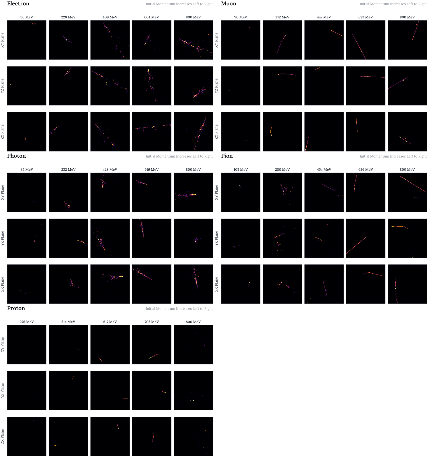
Each event has three detector projections: the XY, YZ and ZX planes. The animation cycles through the five classes. Each frame shows five training events chosen to span the momentum range from lowest to highest.

Heavier particles leave shorter, denser tracks. Lighter particles travel farther and scatter more. Electrons and photons both shower, which makes them hard to tell apart by eye.

Example Tracks by Particle Type

Truth-Level Feature Distributions

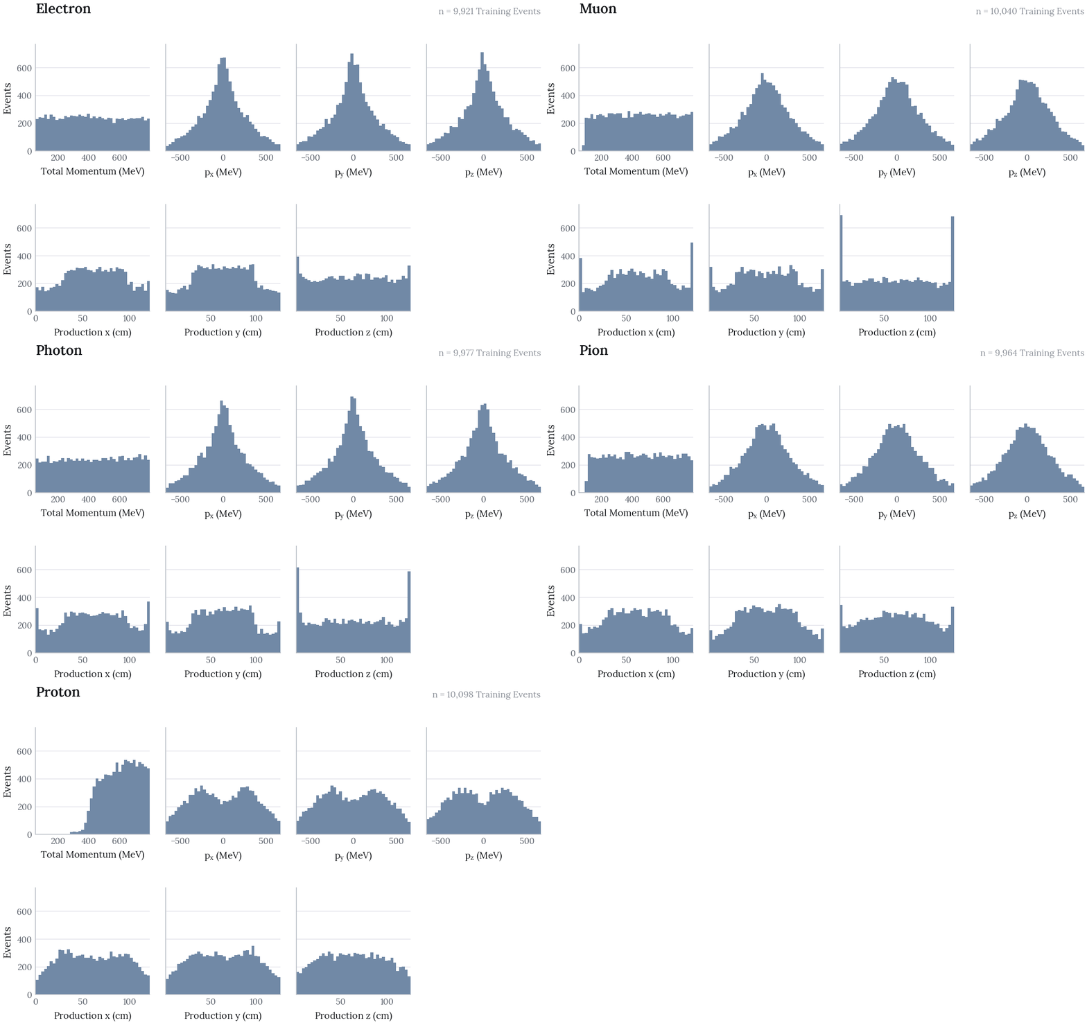
Each image comes with truth-level kinematics: total momentum, its three components, and the production point. The momentum components are symmetric around zero because particles leave in every direction. Total momentum is \(p = \sqrt{p_x^2 + p_y^2 + p_z^2}\) and covers a wide range whose shape depends on the particle type; for protons it starts near 300 MeV and rises. The production coordinates are bounded by the detector volume.

Truth Feature Distributions by Particle Type

Initial Model

Architecture

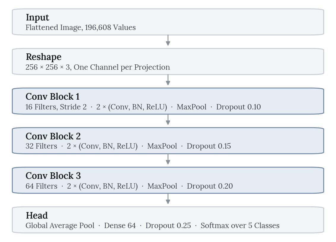
The network has three convolutional blocks. Each block runs two convolutions with batch normalization and ReLU, then max pooling and dropout. The filter count doubles from block to block, from 16 to 32 to 64.

Global average pooling reduces the final feature maps to a single vector. A small dense layer feeds a five-way softmax. The model has about 77,000 parameters, so it trains quickly while still having room to learn the track shapes.

CNN Architecture

Initial Model Performance

Training Dynamics

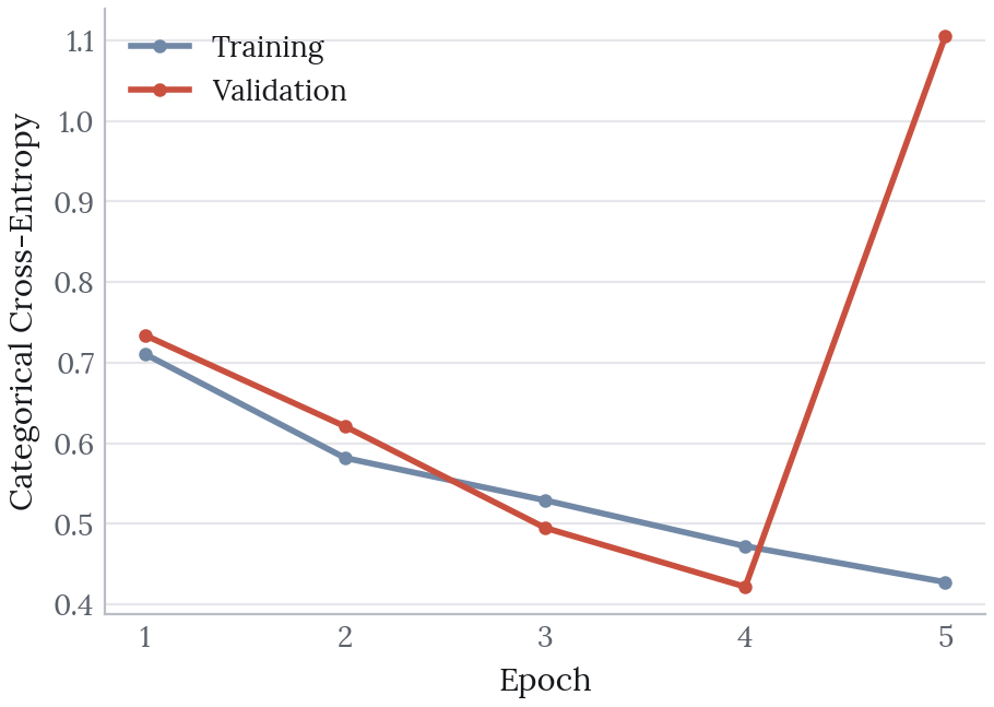
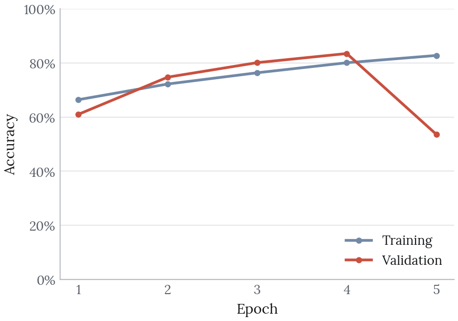
I trained the baseline for five epochs at a learning rate of 1e-3. A plateau scheduler was attached but never fired in that time. Training accuracy climbed steadily to 82.7%. Validation accuracy peaked at 83.4% in epoch 4, then fell to 53.6% in epoch 5. The saved checkpoint is the epoch 4 model, which scores 82.9% on the test set. That swing suggested the learning rate was too high for the model to settle.

Initial Model Loss

Initial Model Accuracy

Classification Performance

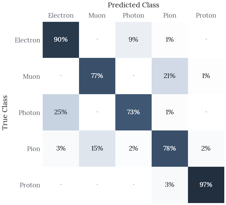
Protons and electrons are the easiest classes, at 97% and 90% recall on the test set. The errors follow the physics. A quarter of photons are called electrons, since both produce showers. Muons and pions leave similar thin tracks, and the model mixes them up in both directions.

Initial Model Confusion Matrix, Test Set. Each row is normalized by true class, and dots mark values under 0.5%.

Hyperparameter Optimization

First Round Results

The first sweep varied one choice at a time against the baseline. Learning rate had the largest effect. Raising it to 2e-3 gave the best validation accuracy of the round, 83.2%.

Wider filters and a larger dense head both made the model worse. Removing batch normalization cost five points. Changing dropout moved accuracy only slightly. Optimization looked like the better lever.

Configuration	Key Change	Best Validation Accuracy	Final Validation Loss
Higher learning rate	Learning rate raised to 2e-3	0.832	0.410
Less dropout	Reduced dropout	0.814	0.462
Baseline	Reference architecture	0.813	0.464
Average pooling	Average pooling in place of max pooling	0.806	0.458
More dropout	Increased dropout	0.790	0.501
Wider filters	More convolutional filters	0.782	0.481
No batch normalization	Batch normalization removed	0.763	0.525
Larger dense head	Wider dense layer	0.759	0.515
Lower learning rate	Learning rate lowered to 3e-4	0.721	0.607

Second Round Results

The second round tested initial learning rates between 1e-3 and 3e-3. The first sweep had used plateau scheduling, which cuts the learning rate when validation loss stops improving. I switched it off here to isolate the effect of the starting rate, then ran each rate again with it switched back on.

Impact of Learning Rate Scheduling

Plateau scheduling improved every starting rate. The best configuration, 1e-3 with plateau scheduling, reached 89.1% validation accuracy. That is 5.7 points above the same rate without it.

Initial Learning Rate	Best Val Acc (No Plateau)	Best Val Acc (With Plateau)	Improvement
1.0e-3	0.834	0.891	+5.7pp
1.2e-3	0.679	0.735	+5.6pp
1.5e-3	0.633	0.820	+18.7pp
2.0e-3	0.654	0.832	+17.8pp
3.0e-3	0.641	0.844	+20.3pp

Final Model

Performance Evaluation

Training Dynamics

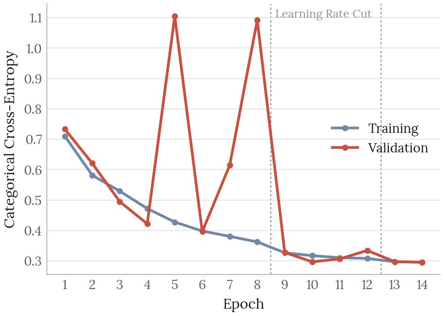
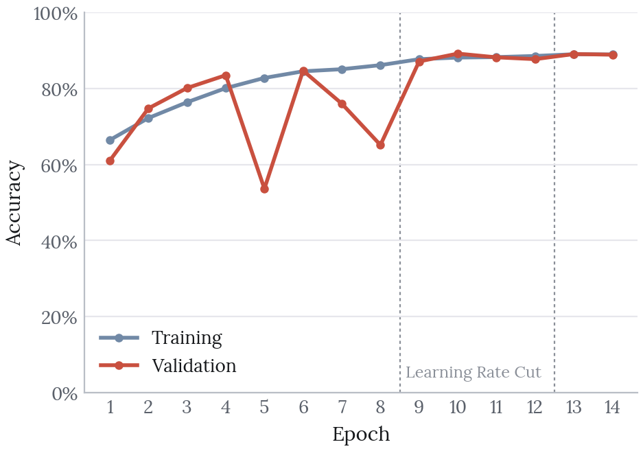
The final model trained for 14 epochs. Through epoch 8 the validation accuracy swung between 54% and 85%. The scheduler then cut the learning rate from 1e-3 to 2e-4 from epoch 9, and to 4e-5 from epoch 13. After the first cut, validation tracked training closely. Validation accuracy peaked at 89.1% in epoch 10, and that checkpoint is the final model.

Final Model Loss

Final Model Accuracy

Classification Performance

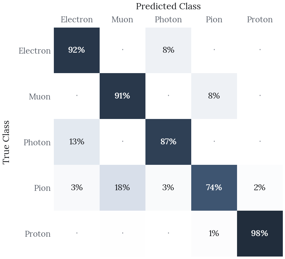
On the 40,000 test events the final model scores 88.2%, up 5.3 points from the initial model. Muon recall rose from 77% to 91% and photon recall from 73% to 87%. Pions did not improve. About 18% are still called muons, and that pair is the main remaining weakness.

Final Model Confusion Matrix, Test Set. Each row is normalized by true class, and dots mark values under 0.5%.

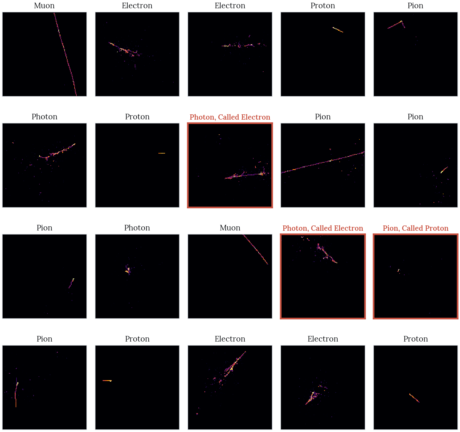
The grid below shows the first 20 test events in the XY plane, unselected. Seventeen are correct. Two of the three errors are photons called electrons.

First 20 Test Events With Final Model Predictions

Next Steps

Architecture. Try residual networks or attention to separate pions from muons.

Evaluation. Add uncertainty estimates so low-confidence predictions can be flagged.

Explainability. Use Grad-CAM to show which parts of each image drive a prediction.

References

[1] MicroBooNE Collaboration. “A Convolutional Neural Network for Multiple Particle Identification in the MicroBooNE Liquid Argon Time Projection Chamber.” arXiv:2010.08653 (2020). https://arxiv.org/abs/2010.08653

Also covered

Machine LearningSupervised LearningConvolutional Neural NetworkKerasTensorFlowHyperparameter OptimizationParticle PhysicsPython

NextMNIST Variational Autoencoder