Olivia Jackson Lambert

Work About Contact

MNIST Variational Autoencoder

A variational autoencoder that squeezes handwritten digits into two numbers and still sorts them into digit clusters without seeing a label.

The Decision

Keep the latent space to two dimensions so that what the model learns can be seen directly.

Takeaways

• Ten digit clusters form without the model ever seeing a label.
• Fours and nines overlap almost completely, and the same pair fails in reconstruction.
• A nearest-centroid rule in the two-dimensional space recovers the right digit 69.8% of the time.

I built a variational autoencoder (VAE) that compresses 28 x 28 handwritten digit images into two numbers and rebuilds each image from those two values alone. A standard autoencoder learns a fixed encoding for each image. A VAE learns a probability distribution over the latent space instead, which keeps the space continuous. New digits can then be generated by sampling points the model never saw.

I set the latent dimension to 2 so the learned structure can be plotted and inspected directly. This is an early project, and two dimensions is a teaching constraint. It caps performance, and in exchange every claim below can be checked against a picture.

Source code: github.com/olivia-jackson-lambert/digit-variational-autoencoder

Data Exploration

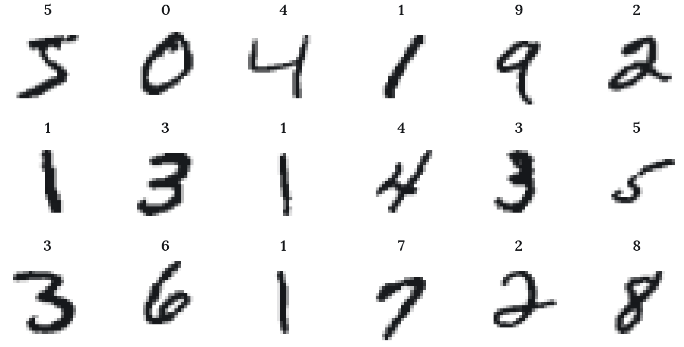
MNIST has 60,000 training images and 10,000 test images of handwritten digits, each 28 x 28 pixels in greyscale. I added a single channel dimension, scaled pixels to the range 0 to 1 and shuffled the training set.

Eighteen training examples with their labels.

Building the Variational Autoencoder

The encoder maps each image to a distribution in the latent space, described by a mean and a log-variance. The decoder maps a point sampled from that distribution back to an image.

Encoder

Input Layer

• Matches the 28 x 28 x 1 image shape.

Convolutional Layers

• 32, 64 and 128 filters give enough capacity for MNIST while keeping the model small.
• A 3 x 3 kernel picks up local stroke features such as curves and junctions without over-smoothing.
• Strides of 1, 2 and 2 shrink the spatial size as the filter depth grows.

Flatten and Dense Layer

• The feature maps are flattened into a single vector.
• A 256-unit dense layer extracts further features before the bottleneck.

Latent Distribution

• Two parallel dense layers output z_mean and z_log_var, the parameters of a Gaussian.

Sampling

The sampling layer draws a point from the encoder’s distribution using the reparameterisation trick:

\[z = \mu + \exp(0.5 \log \sigma^2) \odot \epsilon, \qquad \epsilon \sim \mathcal{N}(0, 1)\]

All the randomness sits in \(\epsilon\), which is treated as an input. The operation stays differentiable, so gradients can flow back through the encoder during training.

Decoder

Input Layer

• Takes the two latent values produced by the encoder.

Dense Layers

• Two hidden dense layers of 256 units each, matching the encoder.
• Dense layers connect every latent value to every part of the rebuilt image.
• ReLU activations expand the representation back towards the original size.

Output Layer

• A 784-unit dense layer with sigmoid activation gives pixel values between 0 and 1.
• The output is reshaped to 28 x 28 x 1 to match the input.

Loss Function

Training balances two terms that pull against each other.

1. Reconstruction loss is binary cross-entropy summed over pixels. It measures how closely the output matches the input.
2. Kullback-Leibler (KL) loss measures how far each encoded distribution sits from a unit Gaussian. It keeps the latent space continuous.

With reconstruction loss alone, the model could place encodings anywhere and leave gaps between them. The KL term closes those gaps, which is what makes the space safe to sample from.

Training

I trained for 50 epochs with a batch size of 128 and the Adam optimiser, validating against the test set.

Loss component	Epoch 1	Epoch 50
Total	188.0	136.6
Reconstruction	183.9	129.6
KL	4.1	7.0
Validation total	167.6	143.4

Loss per image over 50 epochs. The KL term is scaled by ten so it shares the axis.

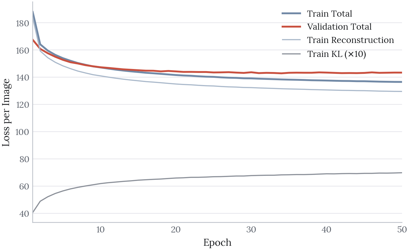
The KL term rises from 4.1 to 7.0 while reconstruction falls from 183.9 to 129.6. The model buys better reconstructions by letting the latent distribution drift further from the prior. That is the trade the two terms exist to negotiate.

Training and validation separate after about epoch 15 and finish at 136.6 and 143.4. Validation barely moves after epoch 25, going from 143.5 to 143.4, so the later epochs mostly improve the fit to the training set. Training could have stopped earlier.

The Latent Space

Digit Clustering

Test digits encoded into the latent space, one colour per digit. Each label sits on its class centroid or points to it with a leader line.

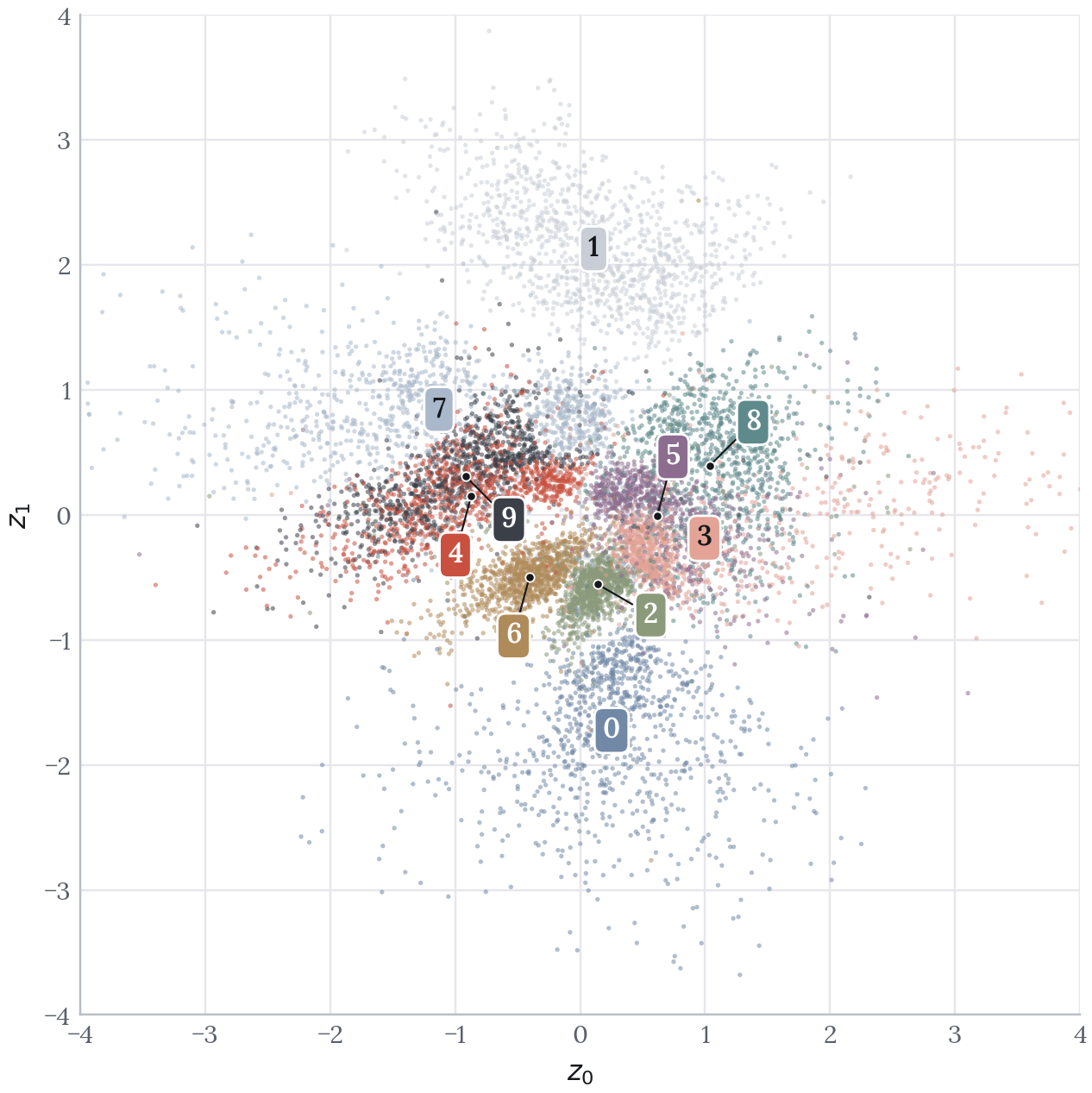
Each digit class occupies its own region of the latent space, and the model never saw a label. The clustering comes entirely from pixel structure.

Some overlap is expected in a VAE. To measure it, I fitted a Gaussian to each class and computed the Bhattacharyya coefficient for every pair.

Digit pair	Overlap		Digit pair	Overlap
4 and 9	0.950		7 and 9	0.671
3 and 5	0.794		2 and 3	0.600
5 and 8	0.740		0 and 1	0.002
3 and 8	0.684		1 and 6	0.002

A coefficient of 1.0 would mean two classes are indistinguishable. Fours and nines reach 0.950. Both are a closed or nearly closed loop above a vertical stroke, and the main difference is whether the loop closes. Zeros and ones share no stroke structure and sit at 0.002.

A nearest-centroid rule in this space recovers the correct digit 69.8% of the time. Chance is 10%, and any supervised classifier would do far better. That gap is a fair measure of what two dimensions can hold.

Reconstruction

The first ten test digits, each input beside its reconstruction from the two latent values. Rust outlines mark the three that come back as a different digit.

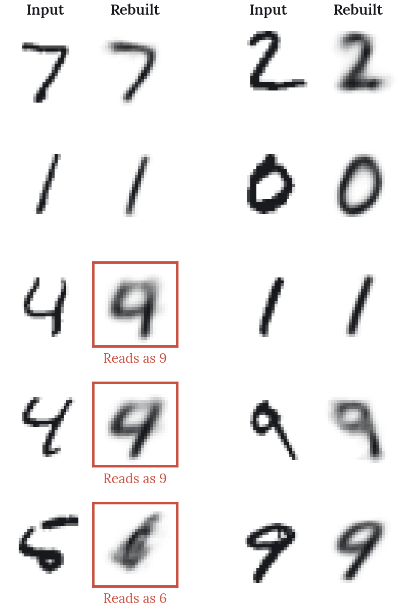
Reconstructions are recognisable but soft, and the failures are the useful part. Both fours come back as nines and the five comes back as a six. Four and nine is the pair the overlap table already flags, now visible in single images.

Generating Digits

Decoding points on a regular grid across the latent space shows what the model has learned.

Digits decoded from an 18 by 18 grid of points spanning −2.6 to 2.6 on each latent axis.

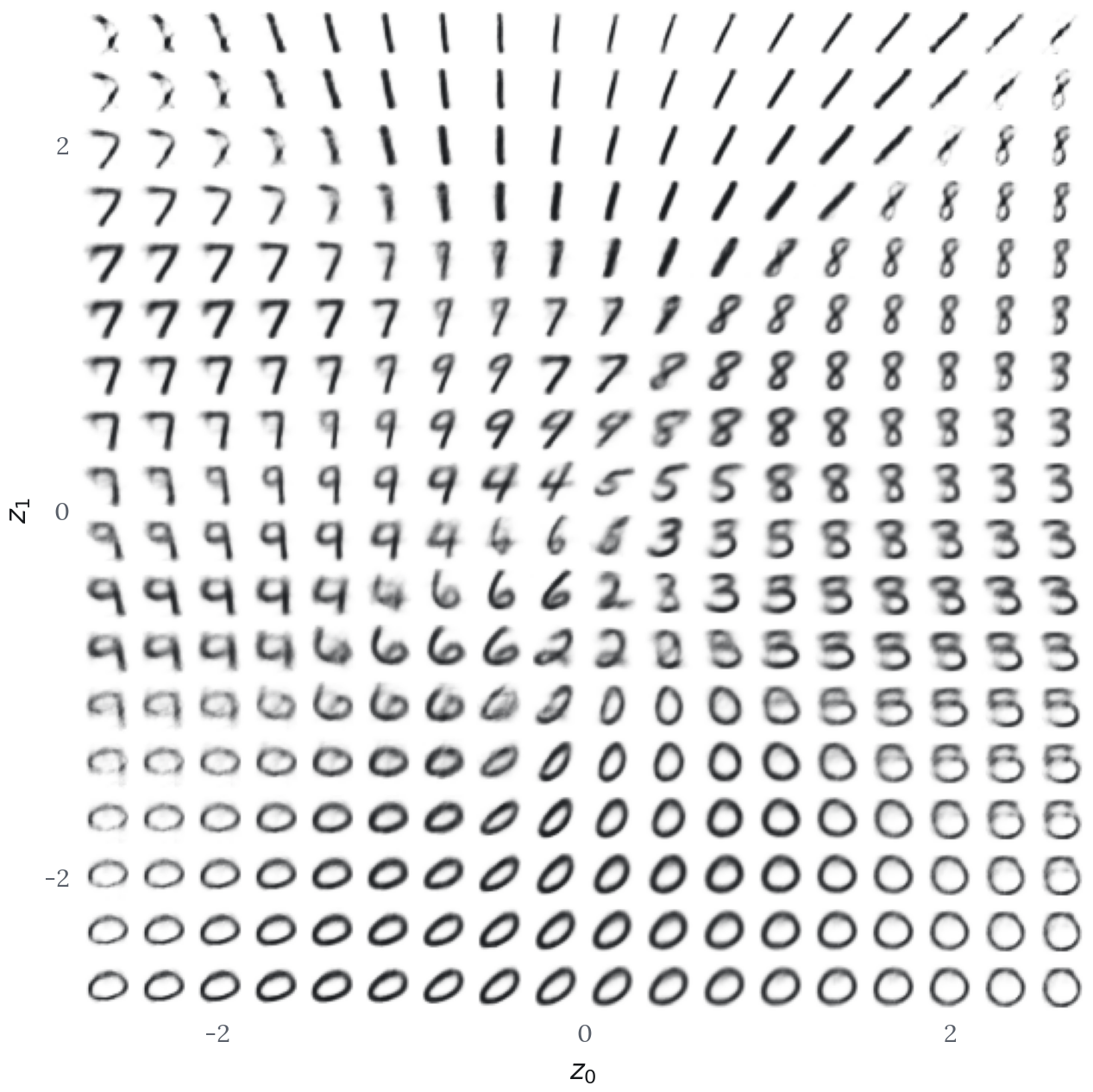
Where classes overlap, the decoded digits sit partway between shapes. Where one class dominates, the digits are sharp, such as the 8s in the upper right and the 0s along the bottom.

Every point on the grid decodes to something digit-like. A standard autoencoder would leave unusable gaps between clusters, so this grid is the clearest evidence that the space is continuous.

A Note on Reproducing This

The original notebook was written in Keras against tensorflow.python.keras, which no longer exists in current TensorFlow, so it cannot run today. The figures here come from a PyTorch re-implementation with the same architecture, loss function and hyperparameters.

The re-implementation lands close to the original. Final training loss is 136.6 against the original’s 138.6, and KL rises from 4.1 to 7.0 against 4.8 to 6.8. The one difference is the gap between training and validation, which the original run did not show. The qualitative findings reproduce, including which digits overlap.

Limitations

Two latent dimensions is a presentation choice. It makes the space directly plottable but caps reconstruction quality well below what a larger bottleneck would reach. The softness in the generated grid comes from that constraint.

Sample quality is judged by eye. Loss values and visual inspection are the only measures. I did not apply a quantitative sample-quality metric.

No baseline comparison. A standard autoencoder with the same architecture would show how much of the smoothness the KL term is responsible for.

Next Steps

Latent dimensionality: Train with more latent dimensions, compare reconstruction loss and use a method such as t-SNE to inspect structure that can no longer be plotted directly.

Conditional generation: Extend to a conditional VAE so a specific digit can be requested directly.

Loss weighting: Vary the weight on the KL term to trace the trade-off between sharp reconstructions and a continuous latent space.

NextPredicting Flight Delay Severity at Scale