Predicting Flight Delay Severity at Scale
In collaboration with Parul Lakhotia, Ewura Impraim Mensah, Roshni Misra and Sarah Son
The Decision
Select the only model that clears the 50% severe-delay recall floor, even at the cost of overall agreement.
Takeaways
- The severe-weighted random forest recovered 64.4% of 2+ hour delays on the 2019 blind test.
- Writing the decision rule down in advance is what made that trade defensible.
- Four model families stall at the same boundary, which points to the features as the limit.
Flight delays cost the US economy roughly $33 billion a year, and passengers bear more than half of it. This project predicts how late a domestic flight will arrive. Each flight goes into one of four ordered tiers, using only information available about two hours before scheduled departure.
The model we selected has the worst overall agreement of our four finalists. We chose it anyway, on purpose, and that choice is the most interesting part of the project.
The Framing Problem
About 82% of flights arrive on time and only 2.2% are severely delayed. A model that predicts “on time” for every flight scores 82% accuracy and is useless to an FAA operator. We rejected accuracy as a success measure before any modeling started.
Instead we pre-registered a decision rule. It shaped the final outcome more than any hyperparameter did.
- Gate 1. Macro F1 above the 0.224 four-class majority floor.
- Gate 2. Recall of at least 0.50 on the 2+ hour tier.
- Models that pass both gates rank on quadratic-weighted Cohen’s kappa (\(\kappa_w\)), which penalizes a three-tier miss far more than a one-tier miss.
- An asymmetric expected cost per flight (ECPF) breaks ties. It charges double for under-prediction, because missing a severe delay costs more than over-preparing for one.
Writing the rule down in advance is what let us defend the final selection later.
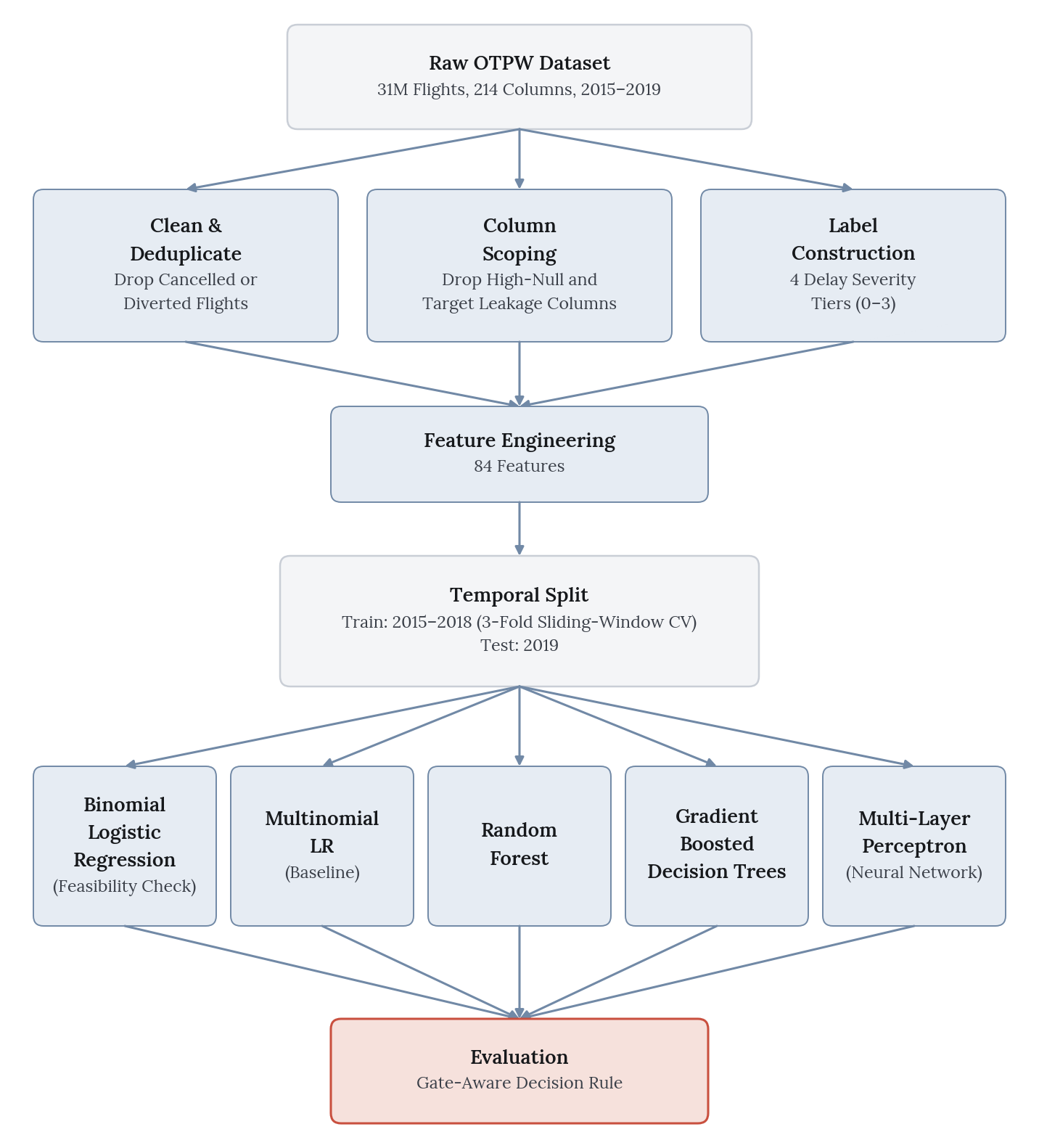
All of 2019 was held out as a blind test set (7.24M flights). The years 2015 to 2018 supported three-fold sliding-window cross-validation, with a one-year training window and a three-month validation window per fold.
Random Forest: Buying Severe Recall
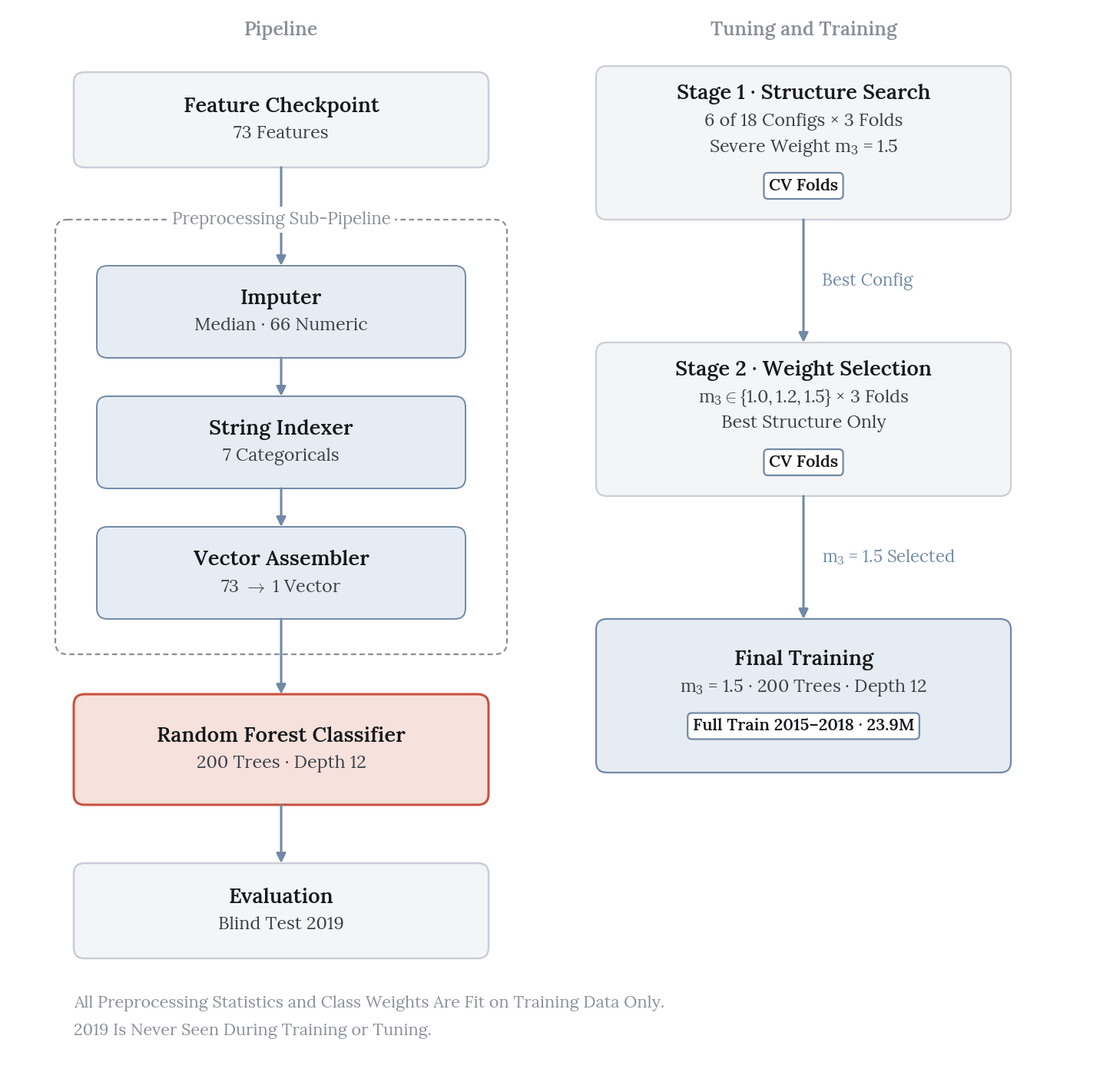
The Phase 2 forest failed Gate 2 badly, at 0.351 severe recall against the 0.50 floor. For Phase 3 the data grew from one year to five (5.7M to 23.9M training flights) and the feature set from 41 to 73 columns. That was not enough on its own, so we added a severe-class weight multiplier on top of standard inverse-frequency weighting.
Staged Search
We ran selection in two stages instead of one large grid. The weight and the tree structure interact, and a single grid would have been slower and harder to read.
Stage 1 fixed the multiplier at 1.5 and varied tree structure. Six of eighteen planned configurations completed before an executor crash halted the deeper trees, so maxDepth 15 and 18 remain untested.
| # | Feature subset | minInst | Val \(\kappa_w\) | Val macro F1 | Val severe recall |
|---|---|---|---|---|---|
| 1 ★ | sqrt | 10 | 0.257 | 0.416 | 0.585 |
| 2 | sqrt | 20 | 0.257 | 0.416 | 0.588 |
| 3 | onethird | 10 | 0.250 | 0.429 | 0.569 |
| 4 | onethird | 20 | 0.250 | 0.429 | 0.571 |
| 5 | 0.5 | 10 | 0.251 | 0.428 | 0.565 |
| 6 | 0.5 | 20 | 0.250 | 0.427 | 0.568 |
sqrt feature subsetting won on both \(\kappa_w\) and severe recall, and it trained fastest. Our reading is that limiting the features each split can see pushes the trees onto the few high-signal propagation features that separate severe delays. With more features per split, the splits spread across weak weather and calendar columns. Leaf size barely mattered. Moving minInstancesPerNode between 10 and 20 changed every metric by 0.003 or less, so the regularization came from bagging and feature subsampling rather than leaf constraints.
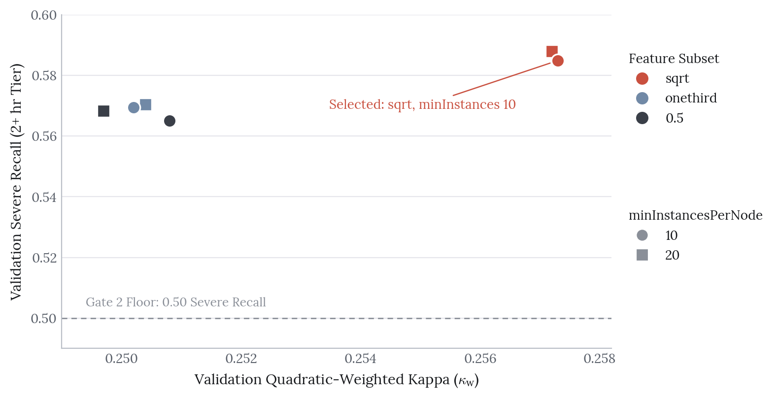
sqrt subsetting sits clearly ahead on both axes.Stage 2 re-ran cross-validation on the winning structure across severe-class multipliers. The result is cleanly monotonic, and it tells the story of the whole project.
| \(m_3\) | Val \(\kappa_w\) | Val macro F1 | Val severe recall | Gate 2 |
|---|---|---|---|---|
| 1.0 | 0.398 | 0.451 | 0.410 | ✗ |
| 1.2 | 0.341 | 0.434 | 0.485 | ✗ |
| 1.5 ★ | 0.257 | 0.416 | 0.585 | ✓ |
Why Cross-Validating the Weight Mattered
On blind-test numbers alone, \(m_3\)=1.2 looks like it passes Gate 2. Its test severe recall is 0.529, with much better ordinal agreement than 1.5 (\(\kappa_w\) 0.336 against 0.241). It would have been the obvious pick.
Cross-validation disagrees. At \(m_3\)=1.2 the validation severe recall is 0.485, below the floor. Validation runs harder than the blind test at all three multipliers, by 0.03 to 0.06 on severe recall. Each fold validates on a first-quarter window, where delays are heavier and more weather-driven than across a full year.
Choosing 1.2 on test evidence would have shipped a configuration that does not reliably meet the operational floor on held-out data. A blind test exists to prevent exactly that.
The Frontier
The selected forest (200 trees, depth 12, sqrt subsetting, 1.5× severe weight) was the only model in the project to clear Gate 2 on the blind test, at 64.4% severe recall. It also has the worst \(\kappa_w\) and the highest expected cost of any finalist.
| Blind test (2019) | \(\kappa_w\) | Macro F1 | Severe recall | ECPF | Gate 2 |
|---|---|---|---|---|---|
| Multinomial LR (hybrid down/up) | 0.438 | 0.394 | 0.418 | 0.848 | Fail |
| MLP (oversample to 25%) | 0.490 | 0.493 | 0.399 | 0.715 | Fail |
| XGBoost (no severe weight) | 0.406 | 0.455 | 0.464 | 0.877 | Fail |
| Random forest (1.5× severe weight) ★ | 0.241 | 0.402 | 0.644 | 1.743 | Pass |
The severe weight has a price under our own cost function. The forest recovers nearly two-thirds of the 2+ hour tier by predicting severe delays for a large number of on-time flights, and the asymmetric cost matrix charges for each one. The multiplier works as an operating-point control. It does not make the model better at prediction overall.
The same trade-off shows up across model families, which is why we read it as a frontier and not a tuning failure. The MLP’s full-rebalance setting reaches 0.489 severe recall, but its \(\kappa_w\) drops to 0.339. The forest traces the same curve across its three multipliers. Four model families plateau at the same boundary.
Gradient-Boosted Trees, and What Went Wrong
We expected XGBoost to beat the forest. It never got a fair trial.
The severe-weighted XGBoost configuration cleared Gate 2 on validation, at 0.534 severe recall. It could never be trained to completion on the full training window. Runs died on driver out-of-memory failures, and the grid stopped after four of eight planned configurations. The XGBoost row above therefore comes from a reduced substitute with no severe weight. It is not the model we would want judged.
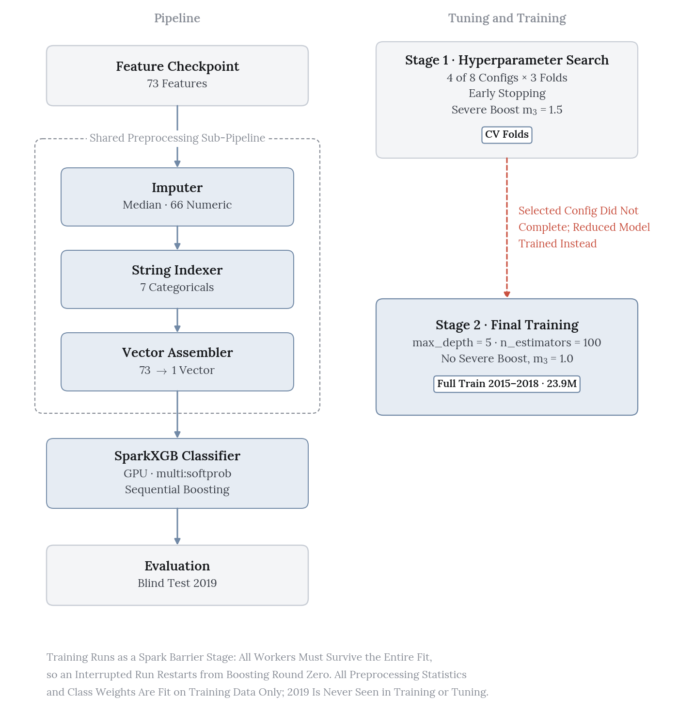
XGBoost remains the most promising unexplored direction. The validation evidence suggests a severe-weighted configuration could hold Gate 2 at higher \(\kappa_w\) than the forest, which would beat our selected model outright. It needs more resilient compute than we had.
That fragility shaped how we ran every search. Executors died mid-grid, so we checkpointed each completed configuration and wrapped fits in retry logic. A crash then cost one configuration instead of the whole run. That is why the random forest grid produced six usable points instead of none.
The Ceiling Is in the Features
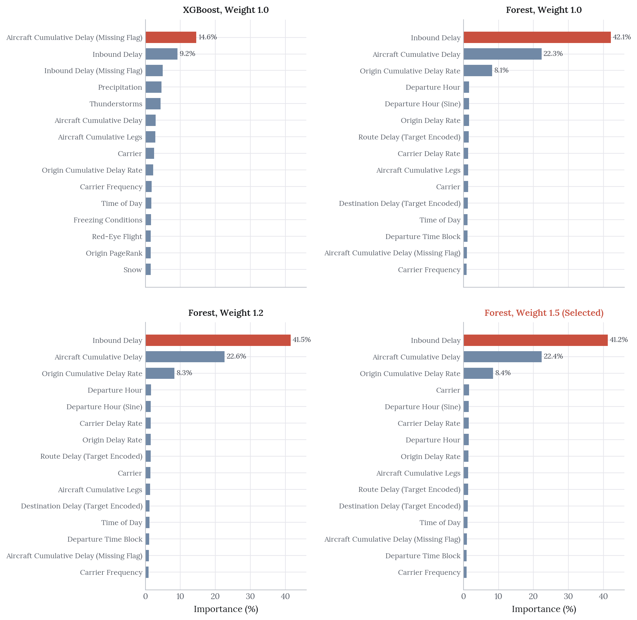
Feature importance is dominated by delay propagation. inbound_delay alone accounts for 41.3% of total Gini importance, tail_cum_delay for 22.4% and origin_cum_delay_rate for 8.5%, about 72% of the model together. Weather contributes roughly 3%, mostly through precipitation.
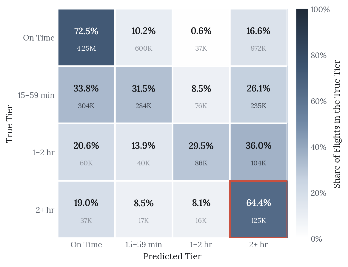
Per-class test recalls for the selected forest are 0.725, 0.315, 0.295 and 0.644 across the four tiers. The middle tiers are the weak spot in every configuration. None of the four tree models gets them above 46% recall, and they fall to about 30% as the severe weight rises. The confusion matrix shows those flights spreading into the on-time and severe tiers more than into each other. Extra severe weight only pulls more of them into the severe tier.
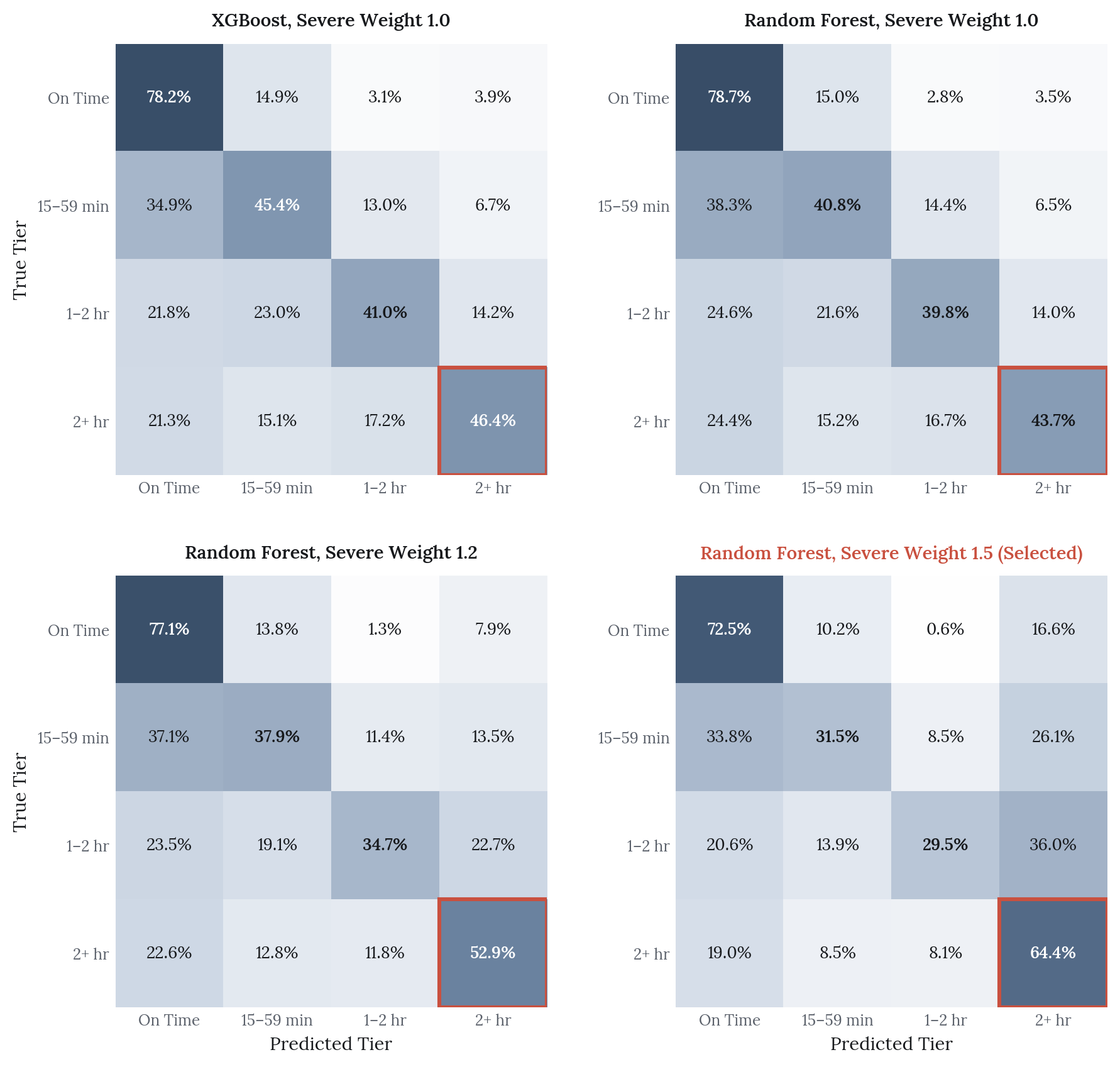
The most plausible explanation is that a 20-minute delay and a 90-minute delay look almost identical two hours before departure. If so, the binding constraint is the feature set, in particular the thin weather and network signal available at that horizon. Model capacity is not the limit. That is useful to know, because it points the next round of work away from bigger models.
Limitations
The search is incomplete. Six of eighteen random forest grid points and four of eight XGBoost configurations finished. All six surviving forest points sit at maxDepth 12, so the selected model may be a local optimum.
The model underfits. Train-to-test \(\kappa_w\) gaps are 0.005, 0.001 and 0.001 across the three multipliers. For the selected model, train and test agree to three decimal places (0.242 and 0.241). That is further evidence that the constraint is signal, not variance.
Phase 3 is not better than Phase 2 on every measure. Severe recall nearly doubled (0.351 to 0.644) while \(\kappa_w\) fell from 0.426 to 0.241. The model is better on the criterion the stakeholder called non-negotiable and worse on overall agreement.
Next Steps
The immediate lever is a cost-sensitive ensemble. A cost-weighted blend of the forest’s severe sensitivity and the MLP’s tier ranking could recover \(\kappa_w\) without giving up the Gate 2 pass. Finishing the forest depth grid and training the severe-weighted XGBoost configuration on more resilient compute would settle whether a boosted model can hold the gate at higher agreement. Longer term, the feature ceiling calls for richer weather signal, such as destination-airport conditions and multi-hour trajectories in place of a single snapshot, more than for extra model capacity.
References
Ball, M. et al. “Total Delay Impact Study: A Comprehensive Assessment of the Costs and Impacts of Flight Delay in the United States.” NEXTOR / FAA (2010).
Data: On-Time Performance with Weather (OTPW), joining U.S. DOT/BTS on-time performance records to NOAA hourly weather observations.